Evolutionary Algorithm
Representation
Coding three ways
Recombination
1-point n-point uniform
Mutation
Selection
Elitism strategies
Computational Models of Gene Regulatory Networks
Computational Models
Boolean Networks
Ordinary Differential Equations (ODEs)
Gene Regulatory Model for Multi-cellular Growth
Three parts, a model for cellular growth, a model GRN model (describing the process of gene expression) controls cellular growth, and an evolutionary algorithm evolving the GRN to achieve the object (the behavior of cellular growth)
Multi-cellular Development Model
Genetics
Gene
Consisting of some SUs and some RUs
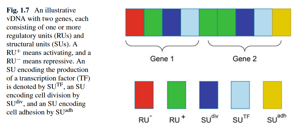
SU —— Structural Units
$\bar{x} = (x_1, x_2, x_3, x_4, x_5)$
$x_1$ determine the action type t
Case t = 1:
Encode a cell division
$x_2$ determine the division angle
$x_3 to x_5$ are not defined
Case t = 2:
Produce a TF
$x_2$ encodes an affinity label assigned to TF $aff_{T F}$
$x_3$ denotes the amount of TF to be released
$x_4$ a diffusion constant
$x_5$ the decay rate
Case t = 3:
Produce adhesion molecules
$x_2$ specify the type
RU —— Regulatory Units
\[\bar{y} = (y_1, y_2, y_3)\]Type: activate and inhibit
The overall activity of the gene is determined by the activating and inhibing values of all RUs of it
In $\bar{y}$:
Cellular Interaction

Using grids to define the size of the body to better simulate the cellular development.
The concentration of the TF in one grid is the same.
Cells interact with each other by reading and releasing TFs, and the concentration is the information.
The diffusion of the TFs?
Cellular Developmental Process
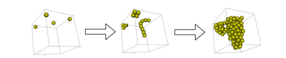
The initial cell (containing the vDNA) in the center area releases a maternal TF, whose concentration is constant. In each developmental step, the vDNA is first translated in all cells.
If the TFs in the vicinity of one cell activate a gene, the action encoded by the gene will be performed. Finally, the position of all cells is updated.
Modeling of Morphological and Neural Development
Modeling Morphological Development
Three reasons to model the biologically plausible morphological development
- Self-stabilized, reach an equilibrium state
- Self-healing
- Generate desired morphology
Design an efficient evolutionary algorithm to evolve the GRN and evolve the cell-cell and cell-environment interactions.
Early Neural Development
GRN-driven
Activity-Dependent Neural Plasticity
Types of Neural Plasticity
- Synaptic plasticity
- Intrinsic plasticity
- Homeostatic plasticity
Hebbian Rules
If neurons are active at the same time, connections between them will become stronger to facilitate further co-activation.
\[\Delta w_i = \eta x_i y_i\]Here the $\Delta w_i$ means the change in synaptic strength, $\eta $means the learning rate, the $x_i y_i$means the pre and post synaptic. And the $\eta $is positive.
Anti-Hebbian Learning
It ensures that the output signals of these cells represent the changes in the input signal in the most efficient way. The formula is the same as above while the $\eta $is negative.
Oja’s Rule
A modification of the plain Hebbian, aim to solve the stability problem of an exclusively potentiating mechanism.
\[\Delta w_i = \eta (x_iy - y^2w_i)\]It represents the self-regulation in plasticity-based learning to make Hebbian-type learning stable.
BCM Plasticity Rules

It’s a rate-based Hebbian rule based on the temporal average of pre- and post-synaptic activity, regulating the post-neuron firing rate to a desired level.
\[\frac{dw_i}{dt} = y(y - \theta_M)x_i - \epsilon w_i\]Here, the $\theta_M$is the regulating parameter. It’s dynamically changed according to $E[y/y_0]$, the $E[\cdot]$ means the average over time, and the $y$is the post-synaptic activity, the $y_0$ is the desired level.
$\epsilon w_i$ is the decay parameter, reducing the connection strength and providing a mechanism for uniform weight decay.
Dual-threshold BCM rule alleviates information loss and enhancing learning performance by introducing different optimal long-term depression thresholds for different post-synaptic neurons.
\[\frac{dw_i}{dt} = y(y - \theta_{LTP})x_i - \epsilon w_i\] \[w_{i}=\left\{\begin{array}{ll}w_{i}+\frac{d w_{i}}{d t} ; & \text { If } y>\theta_{L T P} \\ w_{i} ; & \text { If } y \leq \theta_{L T D}\end{array}\right.\]Homeostatic Regulation
Keep the sum of the synaptic weights connected to a post-synaptic neuron constant.
Any increase in synaptic weight will be balanced out with a decrease in the others.
The synapses are normalized in the following way:
\[w_{ik} = w_{ik}^{'} \cdot N \cdot \frac{w_{avg}}{w_{k}^{'}}\]$w_{ik}^{‘}$ is the weight before normalization connecting from neuron i to neuron k, $w_{ik}$ is the normalized synaptic weight, $w_k^{‘}$ is the sum of all weights fanning into neuron k. $w_{avg}$ is the average weight value of all synapses, N is the number of driving inputs.
Spike Timing-Dependent Plasticity Rules
Depending on the temporal correlation between pre- and post-synaptic spikes.
The synapse between two neurons will be strengthened if the timing of the input spike is slightly earlier than the spike of the output neuron; vice versa, the synapse between two neurons will be weakened if the timing of the input spike is slightly later than the spike of the output neuron.
The stability of the learning can be achieved due to the depressive regions in the learning window.